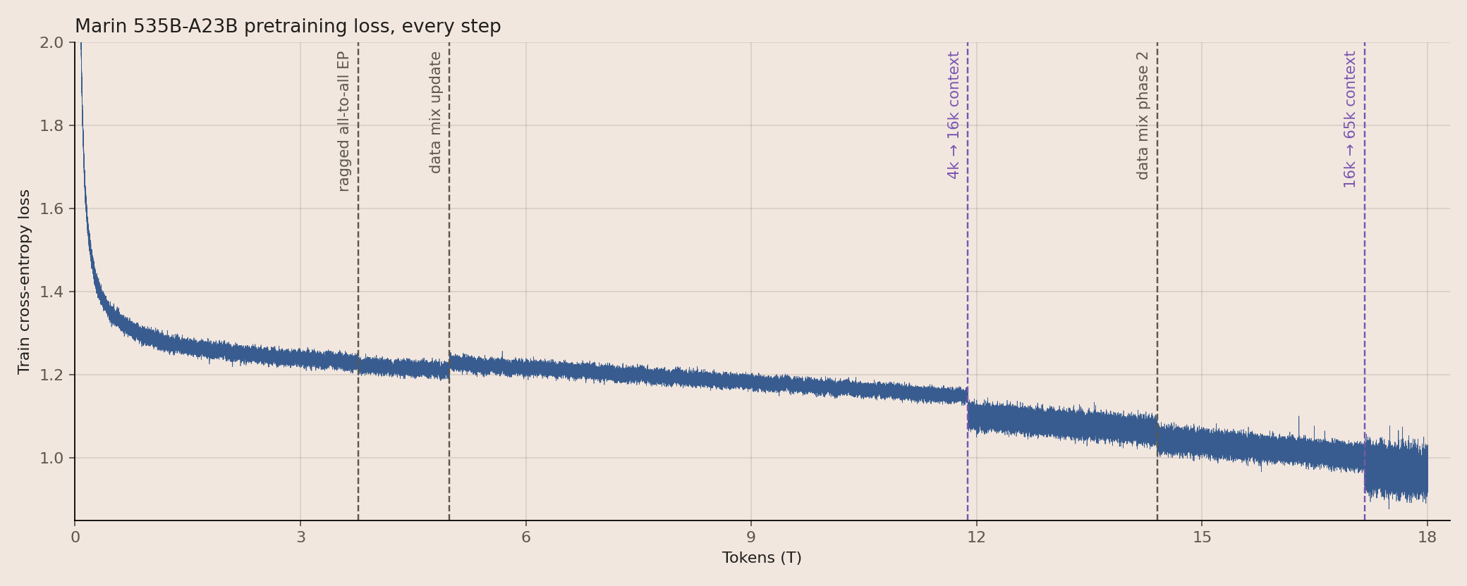
Marin 535B-A23B finished pretraining on 18T tokens on November 5, 2026, representing a big step up in the scale of models Marin has trained. This post is my account of the reasoning and experiments behind its architecture. I first cover the architecture, then how Marin's goals influenced its design, how things were derisked, and evidence behind each component.
Architecture
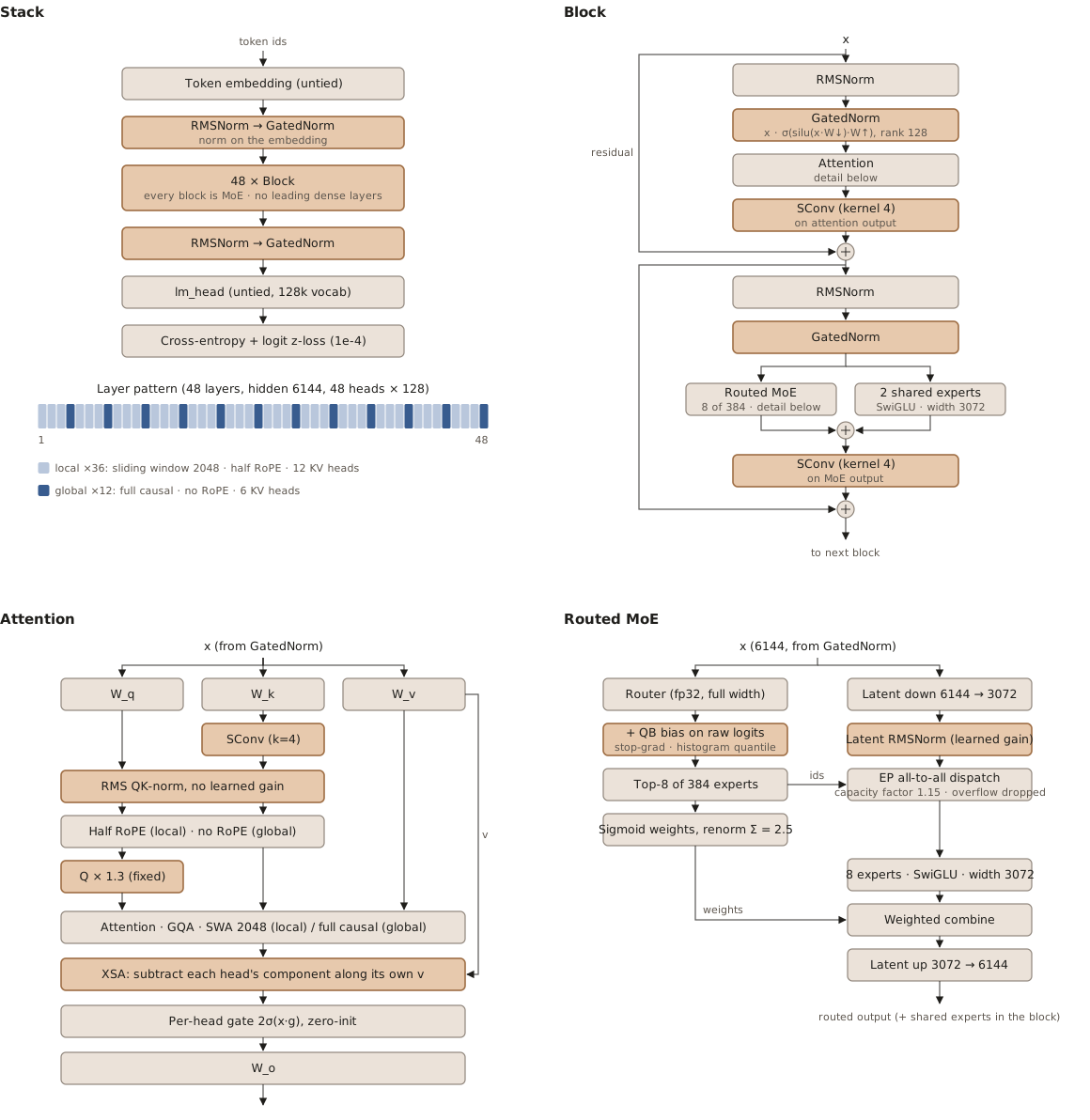
First, the architecture's full details and code can be found here. I'll summarize them below, then afterwards describe how we got here.
Standard components
- 8 of 384 Latent MoE1 (2x compression) with 2 shared experts and SwiGLU activation
- 3:1 local sliding-window (2,048) / global attention, with GQA (4:1 local, 8:1 global) and gated attention2
- Weight initialization with standard deviation 0.5/√
hidden_dim - Sigmoid router; top-k routing weights renormalized to sum to 2.5
- Partial RoPE (50%) on local, NoPE on global
- Logit z loss (weight 1e-4)
- Head dim 128 (num heads =
hidden_dim/128) - Base optimizer Muon3
Notable components
- Learnable RMSNorm on the LatentMoE latent
- Gated Norm4
- Exclusive self attention (XSA)5
- QK RMSNorm with a fixed (non-learnable) 1.3 multiplier
- Short convolutions (SConv) with kernel size 4 on keys, attention output, MLP output
- Top-k Quantile Balancing6 on raw logits, w/ histogram binning for updates
- RMSNorm on the embedding
- 1% warmup, then linear decay to 5% of peak
- Shallow architecture: 6144 hidden dim, 48 layers (width:depth ratio of 128)
- No leading dense layers
- Hyperball7 optimizer: MuonH on all matrices, except AdamH on the
lm_headand plain Adam on the embedding, router, attention gate, norm gains and SConv kernels - LR fit of
adam_lr = 0.087571 · tokens^-0.3461 · hidden^-0.3448 · √(tokens_per_batch), with Adam held at a 3/13 ratio to MuonH (muonh_lr = 13/3 · adam_lr) (fit; see the pretraining speedup post for how the fit is performed)
Background
The design decisions can be best understood through the context of Marin's goals.
The first goal was to make use of 768 GB200s provided on July 15th to produce the best possible model by December, building on the Marin stack in JAX. Out of architecture learning efficiency, realized MFU, and inference speed, realized MFU (different from theoretical MFU) was the dominant driver. That is, every week we were asking, "Will we get a better model by December if we tune model FLOPs utilization for one more week, or if we launch now? What MFU are we actually getting for each architecture feature? How much can we expect to improve MFU mid-run?"
The second goal was to demonstrate that Marin can train large mixture of experts models in a stable and predictable manner. One of the more fun aspects of Marin launches is that for big runs, we preregister a forecast and livestream the run on wandb. This only means something if we put effort into tuning the forecast and launch with an architecture that we have confidence will scale predictably. Achieving this goal is important for enabling future runs.
The third goal was to provide a base for the organization and community to develop supervised fine-tuning and reinforcement learning workflows. To this end, it is useful to launch with an architecture that has similar inductive biases to the literature, such that our first large scale RL runs can leverage prior learnings in the literature. From there, we can branch into more experimental approaches.
Converting these goals into a utility function based on model quality gives something like:
Given that we are in the approaching-the-frontier camp and this run represents our first major scale up, there is substantial utility in minimizing the risk that the run fails or does not complete by December.
Looking for unknown unknowns
The biggest risk on my mind was unknown unknowns: things we are unaware of until they go wrong. To address this, I find it helpful to work in ways that enable surprise. Specifically, getting as much mileage as possible on the hardware in the month before launch, look at a bunch of plots manually, and get exposed to information I wasn't specifically looking for. Here are some issues this uncovered:
- On GPU, every 1/10,000 steps on every 1/10 runs, the
lm_headparameter norm would collapse due to incorrect numerics on a sharded calculation. This was fixed by moving away fromjnp.linalg.normto an explicit norm with an explicit sharding call (Issue #8073).
lm_head parameter norm, which hyperball should hold fixed. At step 24,682 the norm drops from 150.7 to 21.4 in a single update and the loss jumps from 2.07 to 9.14; the gradient was normal at the step that produced the bad update. An earlier, smaller drop at step 4,575 (176.7 to 150.8) is the same bug, with little visible effect on loss. The total parameter norm changes by only 0.24% at the collapse, so the per-matrix norm is what exposes it.- Running without logit z loss on the
lm_headcaused loss blow up in the overtrained regime, so we kept it in the recipe. Even though hyperball constrains thelm_headmatrix, the RMSNorm gain on the activation entering thelm_headwould continue to grow, leading to substantial logit growth (Issue #8227).
lm_head. The two runs track each other until about step 2,500; without z loss the gain keeps growing to 557, versus 183 with it.Building on prior runs
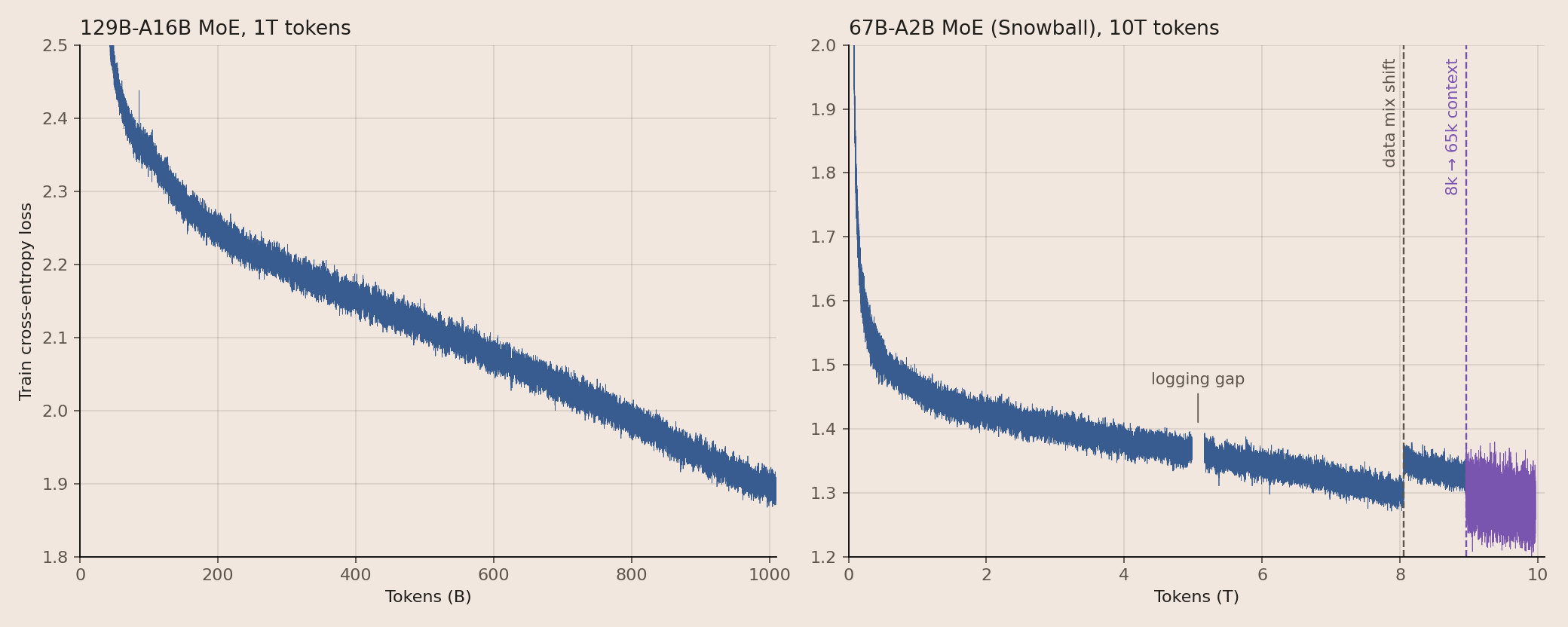
Leading up to this run, we had done two prior MoE runs on TPU: a 129B-A16B MoE for 1T tokens (~1e23 FLOPs) and a 67B-A2B MoE (Snowball) for 10T tokens (~1.2e23 FLOPs). Both pre-training runs landed within 1 percent of their loss target with zero loss spikes. This evidence of stability influenced the design approach for the hero run. Any design that substantially deviated from these two architectures would give up this evidence of stability, and therefore need a higher advantage in other aspects to justify it.
Sizing the model
The model size was influenced by six factors:
- Deadline. We had 768 GB200s and a December deadline, which left ~25 days to get everything running on the hardware and prep the run, ~80 days of training, and 15 days of buffer.
- Pre-train compute optimality. Prior isoflop curves indicated that our MoEs were compute optimal around 60 tokens per active parameter (e.g. 535B-A23B would be compute optimal at ~1.4T tokens). Overtraining by 10x incurs roughly a 2x compute efficiency penalty.
- MFU. GB200s come in racks of 72 GPUs, generally considered healthy if at least 64 are available. Comms are much faster within a rack, so a large MFU hit is incurred if the model cannot fit on a single rack.
- Data availability. We curated 23T deduplicated training tokens. We can run multiple epochs on high quality tokens to increase that, and we also can downsample low quality tokens to decrease that.
- RL. We estimated 2 to 3 weeks of compute for a first pass at RL in December.
- Serving efficiency (deprioritized). We did not explicitly target the intelligence versus model size Pareto frontier, which could have been more strongly targeted by reducing parameter count and increasing token count, or emphasizing distillation. The focus was making the smartest model possible with the available resources, with the main users being researchers learning from the process, ourselves and the broader community in service of future models, and specific domains that show promise during RL. Inference speed still carried some weight, since RL rollouts are inference-heavy.
A more sophisticated approach to sizing was performed by Will Held here. Given where everything landed, the sweet spot roughly corresponds to "fit the biggest model possible on one rack with enough active parameters to take ~80 days."
I started Issue #7201 to track candidate sizes, using a reference 20T token budget to simplify comparisons. Within the first 2 days of the GB200s landing in July, we had our first candidate: a 129B-A15B MoE trained on 20T tokens in 57 days. Within a week, several other candidates landed: a 360B-A23B MoE trained on 20T tokens in 82 days, a 707B-A23B MoE trained on 20T tokens in 99 days (sharded over 2 racks), and a 360B-A21B MoE with MLA trained on 20T tokens in 120 days.
Based on the realized MFU of these candidates, the 360B-A23B MoE trained on 20T tokens in 82 days looked most promising. This was the biggest model I could get to fit on one rack with FSDP. My attempts at jax.lax.ragged_all_to_all seemed too slow to make EP work. Later, Rafal Wojdyla developed a custom fixed-capacity expert parallelism implementation (details) that made a 535B-A23B MoE trained on 20T tokens in 85 days fit. However, it also introduced substantial token dropping from its fixed-size sender and receiver buffers, which required a judgment call. Each of the 64 GPUs in a rack keeps a fixed-size pool for each of the 64 destination GPUs, so tokens can drop in 4,096 sender pools per rack, plus 384 per-expert receiver buffers.
Derisking EP token dropping
Running with an experimental token dropping approach was in tension with our second and third goals for the run, so we needed empirical evidence that it would be worthwhile. Two factors were considered: what is the expected impact on model quality, and what is the expected variance in hero run outcome.
Moving to EP, adding 50% more routed weights, and moving to normalized latent MoE together gave roughly 1.3× compute efficiency (EP is what made the extra routed weights fit), as measured from a scaling ladder from 4e19 to 8e21 FLOPs. From a quality perspective, it was a clear win. But how to estimate the impact on variance?
To do this, Rafal first tuned the sizing and token-capacity factors of the EP candidate, and then I ran several experiments:
- What happens if we eval with token dropping on vs off?
- What happens if we swap to dropless mid-run?
- What happens if we increase context length from 4k to 65k mid-run?
- What happens if we scale up from one rack to four racks?
- What happens to token drop rates as we scale?
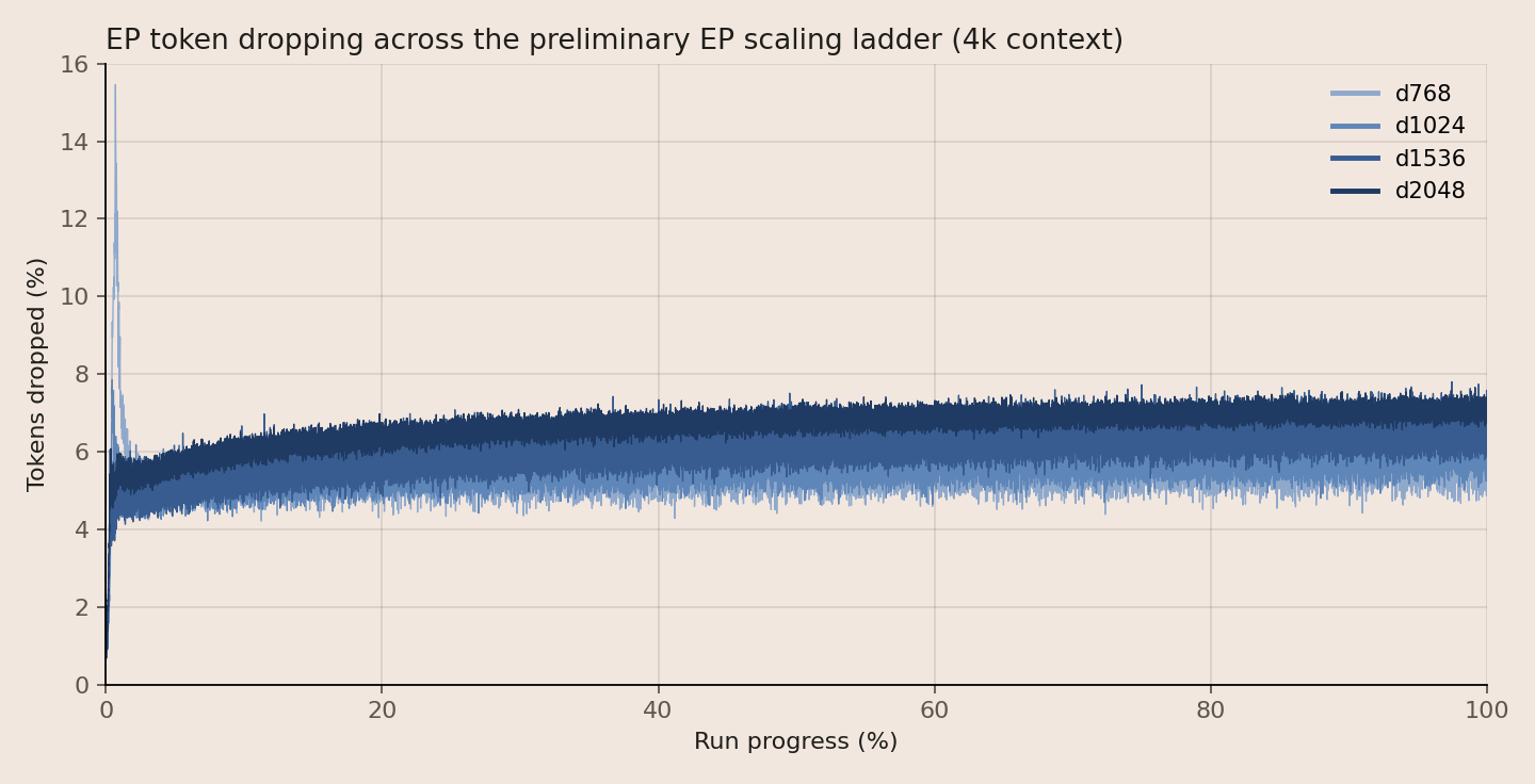
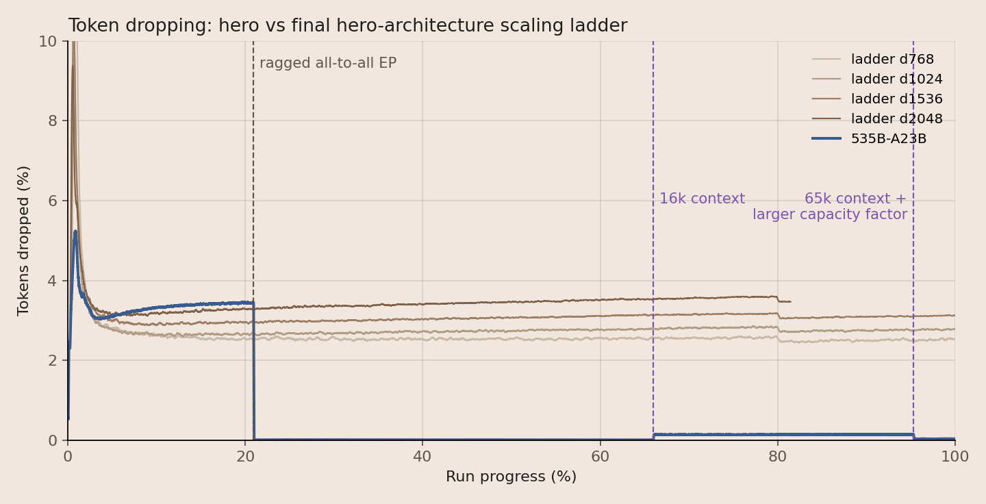
Drop rates crept up slowly with scale, from 5.5% at d768 to 7.1% at d2048 (Figure 8), and scaling the d2048 run from one rack to four racks did not change that trend. Separate small-scale tests showed the model was robust to swapping from small amounts of dropping (~5%) to dropless mid-run.
In the initial small-scale head-to-head, EP's eval loss looked far worse than FSDP's, enough that our scaling law would put FSDP at ~3x more compute efficient. But with token dropping turned off at eval time, EP came out ahead. Routing learns to balance over the train distribution, so a narrow eval like C++ can overload a couple experts and experience heavy dropping. However, since we can run dropless at inference, this concern was moot, and we could focus on the dropless eval number.
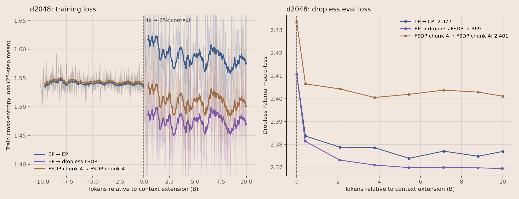
The most compelling evidence that EP would be stable came from the experiment extending context from 4k to 65k. Token dropping jumped from 7% to 37%, yet EP's eval loss landed within 0.01 of switching to dropless FSDP, and all routing metrics stayed stable (Figure 9). I would want to avoid 37% dropping on the hero run, but the stable handling gave confidence that we had a reasonable safety buffer. I care about having a safety buffer because if something unrelated, like a loss spike or a bad data batch, spikes token dropping, I want to avoid a negative feedback loop that blows up the run.
Several decisions were made to further reduce the risk:
- Start the run at 4k context length with the maximum tokens per batch that will fit in memory (46 million tokens). Higher document counts per batch make router balancing simpler, since a large amount of routing variance comes from variance across documents.
- Run with ⅓ of MLP neurons in shared experts, giving a stronger dense backbone in case routing ran into issues.
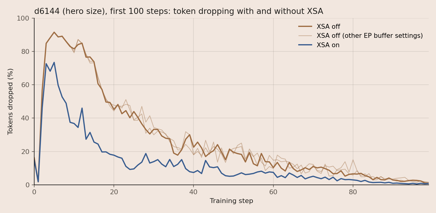
- Keep XSA. XSA improved routing during learning rate warmup.
In the end, the hero's drop rate continued the ladder's trend, until we were able to land a performant ragged-all-to-all kernel and navigate the transition seamlessly mid-run (Figure 10). Thanks to Matt Wittmann for landing it, with some fixes that were later upstreamed to XLA, and to NVIDIA's Sevin Varoglu, author of the device-initiated ragged all-to-all kernel that the EP transport runs on, and Michael Reed for contributing optimizations.
Sizing the scaling ladder
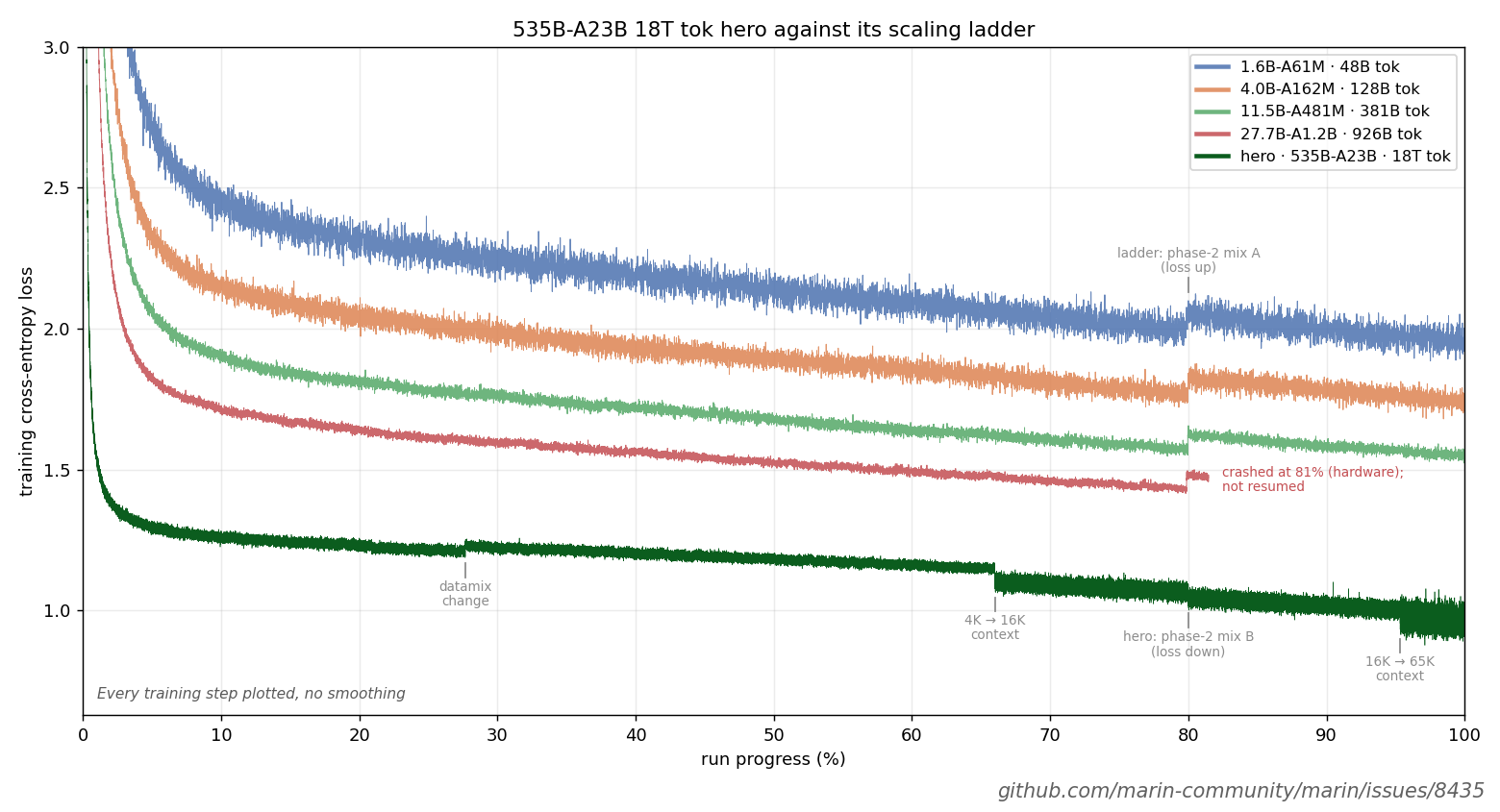
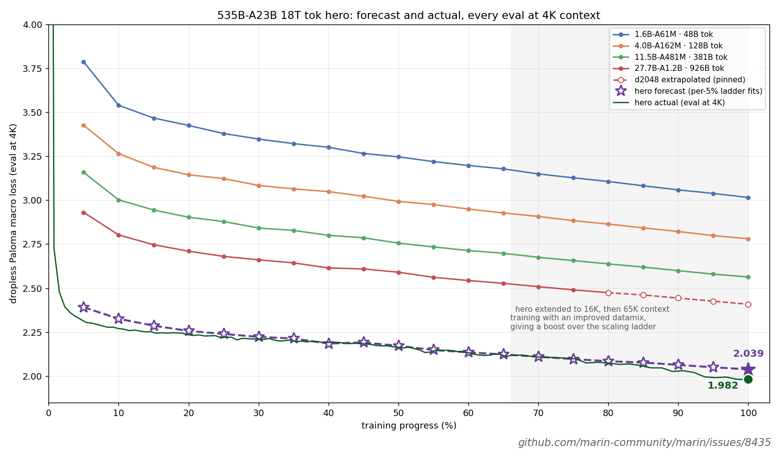
The purpose of the scaling ladder was to confirm our scaling law gave a reasonably low loss projection, catch any abnormal training dynamics, provide a forecast we can track over training, and give us a reference to compare against if we see strange dynamics on the hero run. I ran 4 rungs from 5e19 FLOPs to 9e21 FLOPs, to forecast the hero at 2.7e24 FLOPs, a 300x extrapolation, following our approach from Delphi. The largest ladder rung exactly mirrored the hero batch size in order to simulate EP, multi-rack, and data dynamics accurately.
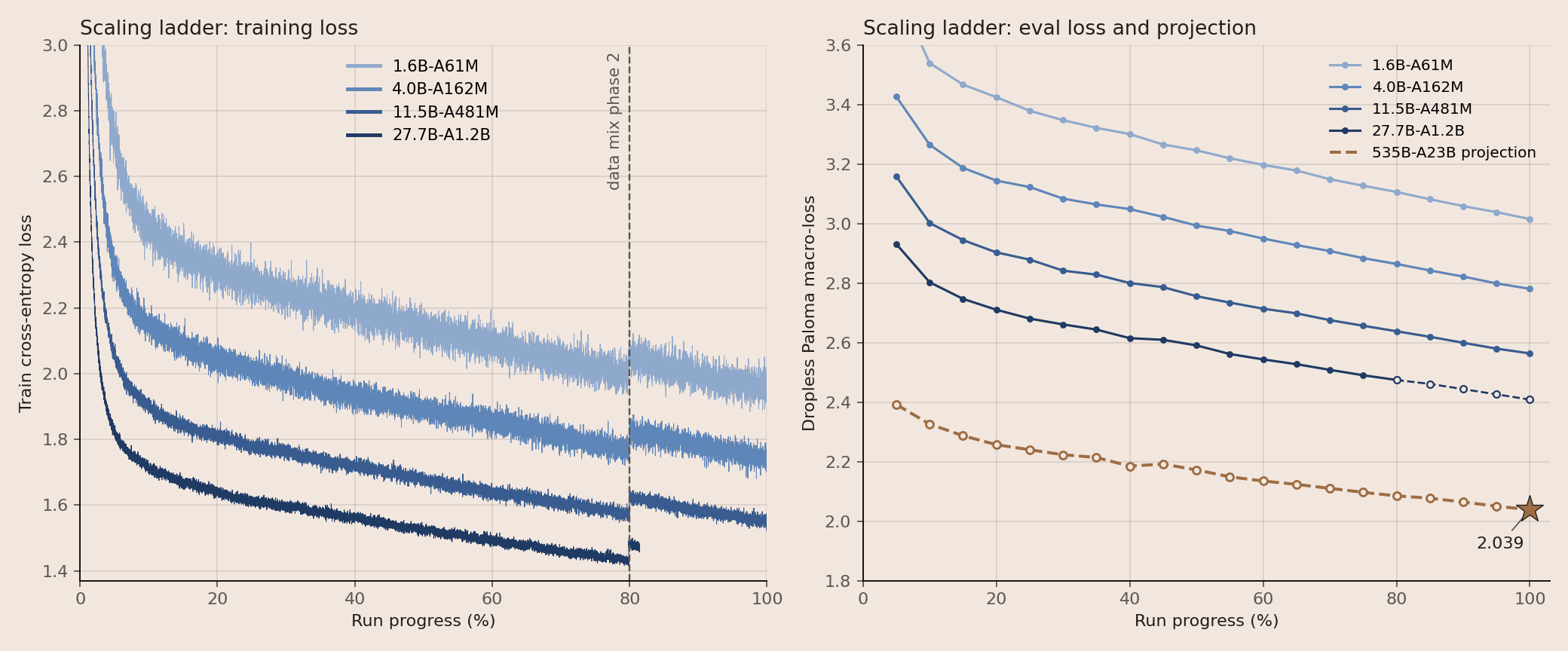
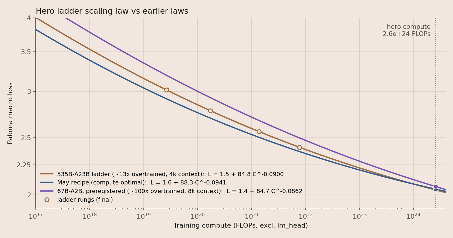
Figure 12 compares the ladder's fit with the two scaling laws we used earlier in the year. This comparison is an important sanity check on the learning dynamics to catch bugs. As expected, at smaller compute budgets the compute-optimal May recipe9 wins, followed by the 13x overtrained hero recipe, followed by the 100x overtrained 67B-A2B recipe. We then see favorable scaling dynamics leading to a lower projection, providing evidence that we aren't incurring substantial numerical failures when shifting from TPU to GPU (both the May recipe and 67B-A2B were trained on TPU).
| Scaling law | Context | Irreducible loss | Overtraining | Hero projection (2.6e24 FLOPs, excl. lm_head) |
|---|---|---|---|---|
| Hero ladder | 4k | 1.5 (calibrated for 4k seqlen) | ~13x | 2.04 |
| May recipe | 4k | 1.6 (initial estimate, set too high) | compute-optimal | 2.05 |
| 67B-A2B | 8k | 1.4 (calibrated for 8k seqlen) | ~100x | 2.07 |
The scaling ladder runs took 2 days, which meant the hero run would have 2 fewer days of compute. An alternative approach would have been to run the scaling ladder for 10 days up to 3e23 FLOPs. My take was that the highest risk portion of the hero run was the first 5 days, with loss blowup as the learning rate ramped, so we'd get more signal from kicking off the hero run itself, rather than running another scaling rung.
Another goal of the largest rung of a scaling ladder can be to pre-screen the SFT and RL process. Given how our run timelines lined up, Snowball, our earlier 67B-A2B run with a similar architecture, was filling this role. As we expand into new architectures without a Snowball-sized cousin to test with, a larger rung on the scaling ladder will be very useful.
Component decisions
The remaining sections cover each architecture component, roughly in the order of the notable components list. Candidate ideas came from recent large releases (Inkling's short convolutions, the sliding window sizes in gpt-oss, Gemma and Trinity), from papers (latent MoE, gated attention, XSA, hyperball), from blogs (quantile balancing), and from our own ablations. Deciding which ideas to adopt followed the stability argument above: the further an idea moved from our two prior runs' architectures, the larger the advantage it needed to show in our ablations, and every idea was then gated on realized MFU on GB200. Throughout, "compute efficiency" is the multiple of compute the baseline would need to match a variant's loss, from our scaling law L(C) = 1.6 + A·C^−0.0941; for example, 1.18× means the baseline would need 18% more compute, and 0.81× means it would need 19% less. It assumes equal throughput, so it does not include MFU differences.
Normalized latent MoE
Initial tests on latent MoE showed surprisingly poor performance, with a compute efficiency of 0.74–0.75 from d512 to d1024 (Issue #6822). Typically when some aspect of the model seems to struggle to learn, the diagnosis method I prefer is to add degrees of freedom with new parameters and observe how the model uses them. Adding a learnable scalar on the latent (a single scalar, initialized to 1, multiplying the down-projected input to the routed experts) showed it climb to about 4 over training, which counteracted the 0.25 scaling induced by initializing the two latent projections to 0.5/√hidden_dim.
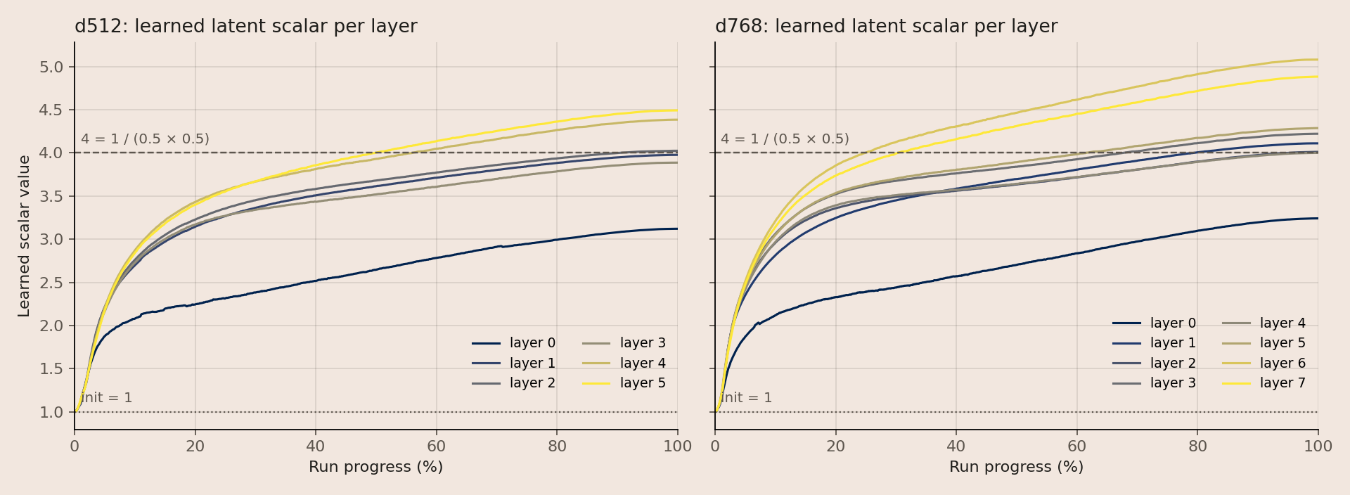
Instead of a learned scalar or updating the init, I found the strongest results from adding a learnable RMSNorm to the latent, taking inspiration from the RMSNorm positioning on MLA. Compared to hyperball with no intervention, this gave 1.25× compute efficiency. This made latent MoE worth including for the MFU gain from halving all-to-all communication.
Gated norm
Gated norm was included in our prior runs to enhance stability, following the advice of Kaiyue Wen. Given how stable those runs looked, there was strong precedence to leave it in. Qwen's Qwen3.8-Next architecture study similarly reports that GatedNorm "markedly improves training stability," and merges it into the Gated Residual design used in Qwen3.8-Flash-Next. We put gated norm in MuonH, based on a comparison of optimizer choices for the gated norm weights.
| Gated norm optimizer | d512 | d768 | d1024 |
|---|---|---|---|
| Adam | 3.7553 | 3.3946 | 3.1392 |
| AdamH | 3.7484 | 3.3835 | 3.1390 |
| Muon | 3.7557 | 3.3895 | 3.1366 |
| MuonH | 3.7471 | 3.3841 | 3.1352 |
Paloma macro loss; all other matrices use MuonH. The differences between optimizers are small (under 0.011) and don't show a consistent trend with scale, leaving open the possibility for further study at larger widths.
Exclusive self attention (XSA)
XSA removes the component of each token's attention output that lies along its own value vector, so attention only carries information from other tokens. In prior recipes we saw a compute efficiency gain from XSA. On the hero recipe, the change is negligible (at d768, removing XSA moved Paloma macro loss from 3.0208 to 3.0221), but we see substantially better router balancing early in training under an accelerated schedule, halving drop rates in the test below.
My intuition is that XSA makes attention start closer to a no-op, so the router inputs change less while attention is still learning (Issue #8227).
I estimated that the biggest risk of the pre-training run would be related to token dropping, so any feature that reduced it was strongly biased towards inclusion. XSA's runtime cost was near-zero.
Microsoft AI used a zero init on the attention output in MAI-Thinking-1 to address this same issue. However, this is not feasible with hyperball, which keeps each matrix at its initial norm, so a zero-initialized matrix would stay at zero. Adding a learned scalar initialized to zero on the attention output seemed like too big of a change to rush through before launch, as it could introduce new LR scaling effects with depth. As a general note on hyperball: in smaller-scale tests, I see that hyperball does not benefit from learned output scalars on the MLP and attention, as long as there is a learnable gain on the input RMSNorm.
QK RMSNorm with a fixed 1.3 multiplier
We see gains from a fixed multiplier after QK norm, as opposed to a learnable per-head scalar.
| Q/K treatment (d768, hero architecture) | Paloma macro loss |
|---|---|
| RMS QK-norm, fixed 1.3 (hero) | 3.0208 |
| RMS QK-norm, learnable per-head gain | 3.0217 |
| RMS QK-norm, no multiplier | 3.0261 |
| No QK-norm | 3.0281 |
At a larger scale (d2048, ~4e20 FLOPs, 60x overtrained), a learnable QK scale also showed no gain: fixed 1.3 ended at 2.6477 Paloma macro loss vs 2.6484 for learnable.
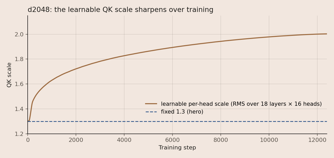
From a risk standpoint, attention logits seem to be a point of failure. The thought is, if we are going to abruptly manually scale up the multiplier during long context extension, as is commonly done with YaRN, then it seems plausible that it should be fixed before then. Absent a larger budget and more experimental cycles to compare long context performance, the decision leaned on the organization goal of producing a stable and predictable run. During the hero run we see clean decreases in loss with no spikes at the context transition points. We scale up the QK multiplier from 1.3 to 1.66 during context extension from 4K to 65K. For 262K, the global layers get a 1.66 base with a log-length query scale, (1 + 0.1·ln(n/65,536))², active from 65K to 262K. This form was tuned directly on the hero via short tests led by Matt Wittmann. This is a squared, floored variant of Inkling's log scaling, in the spirit of SSMax (Issue #8435).
Local sliding window length
Romain Yon measured the inference cost of the attention layout on GB200 with vLLM. Since SWA 2048 was only 2-4% slower than 512 on fixed long-context workloads, we decided to go with a sliding window of 2048. This gave 1.10× compute efficiency at d768 (3.0208 vs 3.0334). While smaller sliding windows seem more common in recent releases (128 in gpt-oss, 512 in Inkling, 1,024 in Gemma 4), Arcee Trinity Large and Command A+ sitting at a 4,096 sliding window provided some external evidence that a larger window gives viable performance at scale.
GQA: 4:1 on local, 8:1 on global
Removing GQA entirely gives roughly 1.2× compute efficiency, but GQA is important to keep to reduce the KV cache at inference. On the hero architecture at d768, full multi-head attention reached 2.9985 Paloma macro loss vs 3.0208 for 4:1 GQA (1.18×).
Since KV heads clearly matter for quality, we kept the local layers at 4:1 GQA rather than reducing them to the 8:1 used on the global layers. The global layers attend over the full context, so their KV cache grows with sequence length and dominates inference memory at long context; that is where 8:1 pays off. The local layers' KV cache is capped by the 2,048-token window, so fewer KV heads there would save little at inference while giving up quality.
SConv on keys, attention output, MLP output
The short causal convolutions were inspired by Thinking Machines' Inkling, which places them after the key and value projections and on the attention and MLP outputs. Each SConv is a learned per-channel convolution over the sequence: with kernel size 4, each output is a weighted sum of the current token and the 3 tokens before it, initialized to the identity and masked at document boundaries. We see a substantial loss improvement from this. Given that our model runs shallow (48 layers vs 60+ in many recent large MoEs), having an additional mechanism for information to flow across tokens seems particularly useful. Within attention, we apply SConv to keys and not values. It is left off values because it gives the smallest gain and blurs XSA: with a conv on values, each token's value mixes in its neighbors, so XSA's removal of the "self" direction would also remove part of the local context the conv adds.
| SConv variant (d1024 ablation) | Paloma macro loss | Compute efficiency |
|---|---|---|
| K, V, attn out, MLP out (kernel 4) | 3.0378 | 1.19× |
| All four sites, kernel 3 | 3.0387 | 1.18× |
| All four sites, kernel 2 | 3.0440 | 1.13× |
| All four sites, global layers only | 3.0482 | 1.10× |
| MLP out only | 3.0506 | 1.08× |
| K only, global layers only | 3.0531 | 1.06× |
| K only | 3.0542 | 1.05× |
| Attn out only | 3.0571 | 1.03× |
| V only | 3.0576 | 1.03× |
| No SConv | 3.0610 | 1.00× |
On the hero architecture at d768, removing SConv entirely cost +0.028 (3.0489 vs 3.0208), while removing only the V conv cost +0.003 (3.0236).
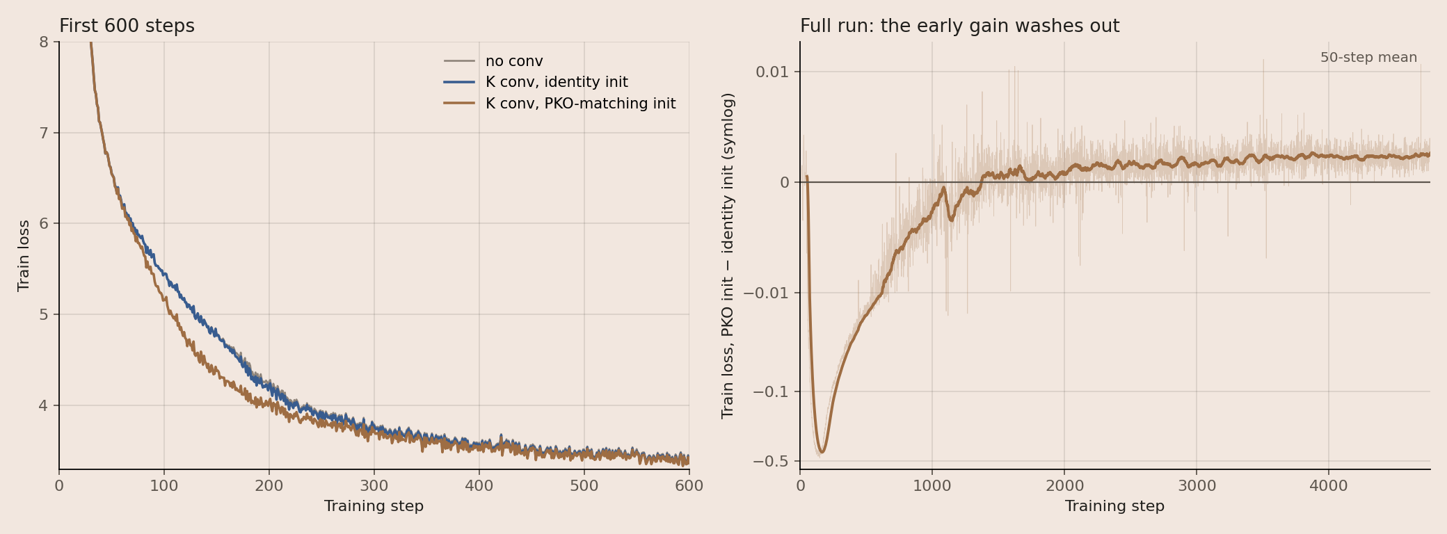
The convolution on keys enables 1-layer induction heads. I tested initializing the K conv to mirror partial key offset, which enables the induction heads to form faster. However, the gains from init wash out over the course of the run, so identity init is kept.
Top-k quantile balancing on raw logits
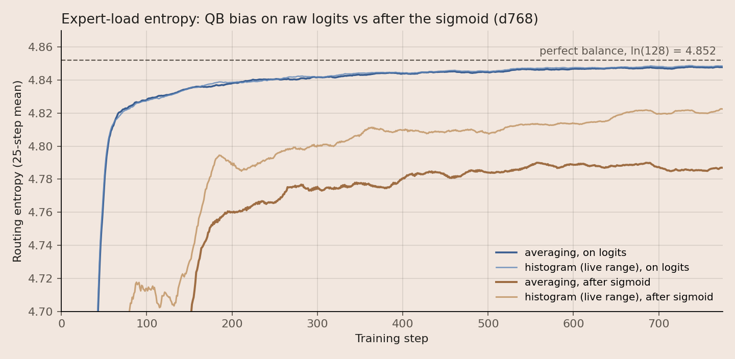
We integrated quantile balancing, from Jianlin Su's blog, into the recipe back in April. (See also our post on the subject.) For this hero run, to keep our implementation independent of GPU count, we use histogram binning instead of averaging per-GPU quantiles, similar to Kimi K3. One key difference: Kimi K3, like DeepSeek-V3, applies the bias after the sigmoid, while we apply it to the raw logits. While the sigmoid gives the histogram a clean 0 to 1 bound, we see substantially faster balancing from logits in our experiments (Figure 17). This is particularly relevant for us due to our nonzero token dropping. Estimating the bin range live with 10,000 bins runs quickly, with no noticeable MFU hit, which removes the need for a clean bound.
The histogram estimators match averaging on loss while balancing slightly better and staying independent of GPU count.
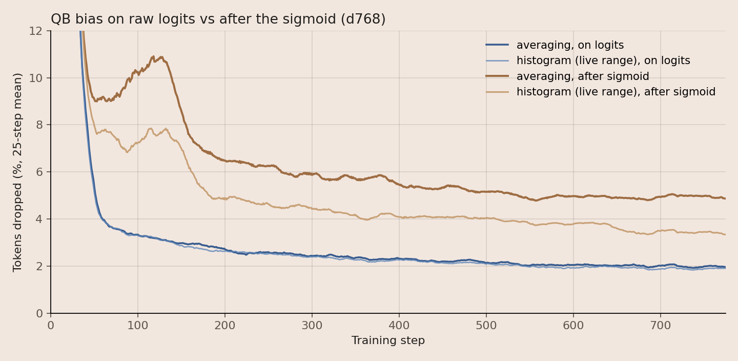
All of the QB variants balance quickly compared to auxiliary-loss methods (earlier post); even a routing entropy of 4.76, against a maximum of 4.852, is already quite good. The last margins matter here specifically because of our token-dropping capacity factors.
Expert granularity
Scaling from 4 of 192 to 8 of 384 shows 1.13–1.16× compute efficiency. Doubling again to 16 of 768 shows diminishing gains over 8 of 384, which did not justify its throughput cost, so granularity was kept at 8 of 384. 8 of 384 with 2x latent compression has a secondary benefit in this config, as it keeps the routed expert matrices square. On square matrices, Muon's orthonormalization step balances the update over both incoming channels and outgoing neurons. This avoids the imbalanced per-neuron updates, and in the extreme the neuron death, that approaches like NorMuon10 and Aurora11 were made to address in rectangular matrices. In an ideal world we would be able to test each of these changes under much larger scaling ladders, but given finite timelines and compute, I rely somewhat on judgment and on external validation, such as the 8 of 384 expert granularity of Kimi K2.
| Routed experts | Expert width (d768) | Paloma macro loss, d768 | Paloma macro loss, d1024 |
|---|---|---|---|
| 4 of 192 | 768 | 3.0289 | 2.7810 |
| 8 of 384 (hero) | 384 | 3.0091 (1.16×) | 2.7674 (1.13×) |
| 16 of 768 | 192 | 3.0009 (1.23×) | not run |
Step-matched runs; compute efficiency vs 4 of 192 in parentheses.
RMSNorm on embed
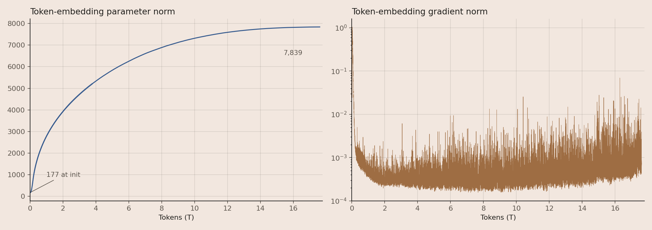
The token embedding is kept outside hyperball, so under Adam its norm grows freely, from 177 to about 7,800 over the hero run (Figure 19). An RMSNorm after the lookup keeps its output at unit scale regardless, matching the forward pass behavior of μP12. As the norm grows, Adam's updates shrink relative to the weights, which acts as a built-in learning-rate decay on the embedding (Issue #4569). In a d768 ablation, removing the embedding normalization cost about 19% in compute efficiency.
Hyperball on lm_head
All Adam parameters are excluded from hyperball, except for the lm_head. The lm_head was tested under AdamH, Cautious AdamW, AdamW, and plain Adam. At very small scale, Cautious AdamW performs marginally better. However, as we scale up, AdamH beats Cautious AdamW with 1.08× compute efficiency (Issue #8350). I note that this does not imply AdamH on the lm_head is strictly superior to Cautious AdamW. Everything in ML is conditional. In particular, in this case the LR recipe was previously tuned on AdamH. However, given limited compute, the 1.08× gap and prior stability evidence of AdamH were sufficient to push compute towards more pressing ablations. Pinning the lm_head norm does not fix the logit scale: the learnable RMSNorm gain on the final activation, trained with Adam, is free to grow and scale up the logits. This is why logit z loss remained necessary.
Linear LR decay
We use 1% warmup followed by linear decay to 5% of peak. Warmup is not necessary under Muon, but we kept it for initial routing stability.
Linear decay beat WSD in our d768 schedule sweep, which I attribute to hyperball. Without hyperball, parameter norms grow over roughly the first half of training, which decays the effective learning rate even during a WSD stable phase. Hyperball fixes those norms, so the decay has to be built into the schedule itself. This is also what gives the straight-line loss curves in Figure 7.
The same sweep tested a 1−√ decay, where the learning rate follows 1−√(t/T) over the run (t is the current step, T the total), dropping faster than linear early and flattening toward the end. It came out slightly ahead (3.2642 vs 3.2670), but only at 1.4× the peak learning rate. That gain was not worth launching at a higher learning rate without further testing, since a higher learning rate could cause issues during the first 3% of the run, the highest-risk point.
Shallow architecture
The hero model is 6,144 wide and 48 layers deep, a width-to-depth ratio of 128. The main reason is MFU: fewer, wider layers run more efficiently on our stack. A secondary benefit is lower risk. We did not add depth-related enhancers such as attention residuals13, mHC14 or skip connections, because I could not make them run efficiently in time. Without them, there is a risk that a very deep network cannot make full use of its parameters. Command A+, with 32 layers, showed that high depth is not necessary for a viable model, so from a derisking perspective a shallower network seemed like the stronger choice.
No leading dense layers
When we moved to quantile balancing, we removed the leading dense layers, since routing entropy in the first layers looked very healthy without them and higher sparsity can increase compute efficiency. Given the move to EP and the related risk from token dropping, there was a case for revisiting this. However, I was not able to get heterogeneous layers working cleanly with jax.lax.scan with a small memory profile in time to pursue it further (certainly just user error on my end).
Preliminary results
Below are the loss curve and scaling projection results for the pre-training run. We will still need to see where the final results shake out after evals, which will be covered in a future report, but the tracking of the loss forecast looks quite promising when compared on a FLOPs vs loss basis to other recent large-scale MoEs (comparison).
Open questions and further considerations
In LLM research there is always an infinite list of open "what ifs" to pursue, which is part of what makes the process fun. Some areas that I would be interested to explore, or see results from others on, leading up to future runs, to improve inference efficiency, scaling efficiency, learning dynamics, and long context:
- Quantile balancing during data mix updates. Quantile balancing rapidly rebalances in 1–2 steps, potentially sending tokens to experts they have never seen before. It seems plausible that a more gradual mechanism could be useful in the event of data mix changes. I would be interested to quantify the impact of rapid bias updates during substantial shifts in data mix, and explore alternatives between the two extremes of freezing biases and enabling 1–2 step full rebalancing.
- Smaller local windows early in training. It may be preferable to start the local SWA layers at a very small context, such as 128, to force the global layers to specialize in long-context retrieval. The current size of 2,048 performs best on perplexity evals for a base model trained at 4–8k context, but it is unknown how this extends to longer context. A middle ground would be to start local layers at 128 and only extend to 2,048 after role specialization is achieved.
- Learned per-head QK multipliers. The fixed QK multiplier is manually extended during context extension. It seems conceivable that the variance across heads from a learned per-head multiplier could give stronger retrieval at long context. Collecting evidence for or against this hypothesis would be useful.
- Final learning rate. Linear LR decay showed the strongest performance when decaying to 0, but we stopped at 0.05 to leave room for SFT and RL. Given the success of checkpoint weight averaging, an even higher final LR may be preferred.
lm_headscaling. Thelm_headshares the standard 0.5/√hidden_diminit and the empirical LR fit's width exponent (LR ∝hidden_dim^−0.345) with the rest of the Adam group. No experiments thus far to steelman μP or its variants have yielded stronger results, and all scaling appears stable under the current config, but it's plausible that at very high widths a 1/hidden_dimoutput scale would be helpful. As compute allows, stress testing this at very wide widths would be useful.- MFU-gated features. We see strong results from a combination of KDA15, attention residuals13, MLA16, and relative position embeddings17, but gate their inclusion on acceptable realized MFU. This is a particular constraint for our org because we are training compute-bound and want to keep our hero run cycles from taking too many months. In the last two months, we see substantial gains in agents' ability to close the gap between theoretical and realized MFU (Issue #9451), making these features more practical going forward.
- FP8 and NVFP4. Given the particular risk profile of this run, we postponed FP8 and NVFP4 training, deeming the speedup not worthwhile given we were already at 20% and later 30% MFU.
- Over-encoding hashed embeddings. We avoid over-encoding18 hashed n-gram embeddings due to realized MFU and memory considerations, though the behavior of n-grams under a changing data distribution or multi-epoching is a further complication that may be suboptimal when building our first large scale RL recipe.
- High depth stress testing. The hero run exhibited different behaviors along depth than the scaling ladder, indicating that it could be useful to stress test a narrow but deep model prior to a large scale run. This is an update we will incorporate into future hero runs, likely based on attention residuals.
- Gated norm optimizer group. Muon performs strongly for near-square matrices. As
hidden_dimgrows, the ratio ofhidden_dimto the low-rank 128 gated norm skews, which may start to favor Adam at large sizes. - Feedback from post-training and richer evals. At this stage, architecture decisions are largely made based on pre-training loss, stability considerations, and how prevalent a component is in existing models. As our future architectures become more opinionated, we will be able to lean less on that prevalence, and will need stronger feedback signals from SFT, RL, and evals that correlate with agentic RL to optimize our pre-training recipe.
- Multi-token prediction. We avoid MTP19 due to memory constraints, realized MFU, and the growing success of separate drafter modules like DSpark20.
- Dead routed experts in initial layers. On the hero run, the routed experts in the first two layers receive abnormally small gradients and likely contribute little, matching what Mooler0410 found in ultra-sparse MoE training, where a temporary aux loss on the first MoE layer early in training kept those experts learning. The problem may resolve in a future architecture with attention residuals, but it is something that should be tracked closely and perhaps handled with an early aux loss.
- Decision making. Part of the goal of articulating all my thoughts on these decisions is to help myself (and others) upskill our decision making process. Hopefully I can look back in a year and see a bunch of things I'd improve, both in terms of making the best decisions given the available information, and knowing what missing information should be collected.
Acknowledgements
This work is generously supported by the Jen-Hsun and Lori Huang Foundation, which provided the compute for this run. The Google TPU Research Cloud program enabled our earlier runs, which built confidence in the recipe.
On architecture leading up to the run, I thank Rafal Wojdyla for his clarity in pursuing EP, which delivered a substantial 1.3× compute efficiency; Mark Muchane for his cross-entropy kernel precision fix, which may also have helped run stability; Kaiyue Wen for his advice on hyperball, gated norm for stability, and architecture dynamics; and Will Held for being a brainstorming partner on architecture ideas. I thank the NVIDIA JAX team for their support in helping us get up and running quickly. I also thank Percy Liang for his vision and strategy in building toward this run. Making this run possible required critical contributions across the entire Open Athena team on infra, data, partnerships, software stack, ops, mid-run MFU boosts, and team coordination, which will be highlighted in a future report.
Elango et al., LatentMoE: Toward Optimal Accuracy per FLOP and Parameter in Mixture of Experts, 2026.↩
Qiu et al., Gated Attention for Large Language Models: Non-linearity, Sparsity, and Attention-Sink-Free, 2025.↩
Keller Jordan, Muon: An optimizer for hidden layers in neural networks, 2024.↩
Qiu et al., A Unified View of Attention and Residual Sinks: Outlier-Driven Rescaling is Essential for Transformer Training, 2026.↩
Zhai, Exclusive Self Attention, 2026.↩
Jianlin Su, Quantile Balancing.↩
Wen et al., Fantastic Pretraining Optimizers and Where to Find Them — Hyperball Optimization. MuonH and AdamH are Muon and Adam with the hyperball projection.↩
dN denotes a model with hidden dimension N; the 535B-A23B hero is d6144.↩
Our May 2026 MoE baseline (PR #6153): 256 experts with 4 active, MuonH, partial RoPE, sliding window 2048, and no z loss, trained compute-optimal on TPU v4. Its compute-optimal fit, L(C) = 1.6 + 88.90·C^−0.0941, is the scaling law used for the compute efficiency numbers throughout this post.↩
Li et al., NorMuon: Making Muon more efficient and scalable, 2025.↩
Tilde Research, Aurora: A Leverage-Aware Spectral Optimizer, 2026.↩
Yang et al., Tensor Programs V: Tuning Large Neural Networks via Zero-Shot Hyperparameter Transfer, 2022.↩
Kimi Team, Attention Residuals, 2026. Our test: Issue #5110.↩
Xie et al., mHC: Manifold-Constrained Hyper-Connections, 2025.↩
Kimi Team, Kimi Linear: An Expressive, Efficient Attention Architecture, 2025. KDA is Kimi Delta Attention.↩
DeepSeek-AI, DeepSeek-V2: A Strong, Economical, and Efficient Mixture-of-Experts Language Model, 2024.↩
Huang et al., Over-Tokenized Transformer: Vocabulary is Generally Worth Scaling, 2025.↩
Gloeckle et al., Better & Faster Large Language Models via Multi-token Prediction, 2024.↩
DSpark: Confidence-Scheduled Speculative Decoding with Semi-Autoregressive Generation, 2026.↩
Cite this post
@misc{dial2026_marin_535b_architecture,
  author = {Dial, Larry},
  title = {Architecture Decisions for Marin 535B-A23B},
  year = {2026},
  month = {nov},
  howpublished = {\url{https://www.openathena.ai/blog/marin-535b-architecture/}},
  note = {Open Athena Blog}
}