This post highlights Quantile Balancing (QB), a load balancing method for Mixture of Experts (MoE) models developed by Jianlin Su. The Marin team validated QB on a 32B total 5B active-parameter (32B-A5B) model trained on Marin infrastructure over 326B tokens (1e22 FLOP compute budget). In this post, I will get into our motivation for using the MoE model family, explain why load balancing is necessary, survey prior approaches to balancing, and share performance results for QB.
Summary
- QB is a hyperparameter-free MoE load balancer from Jianlin Su.
- The Marin team validated it at 32B-A5B / 1e22 FLOPs over 326B tokens on Marin.
- The model run showed zero loss spikes and didn't need leading dense layers or auxiliary losses to achieve balancing.
- This outperforms our prior fixed-increment-bias + aux-loss setup at 1e21.
Why use MoEs?
The short answer is that they empirically work. The following provides intuition for why that is the case, although the real picture is more nuanced1. Large language models are composed of millions of neurons that work together to build a prediction. The mathematics of a single neuron can be loosely understood as a noisy IF-THEN operation. If properties (A, B, C, ...) exist in the current prediction, then activate and write properties (X, Y, Z, ...). For instance, if (Michael, Jordan) exists, then write (Basketball, Bulls). In practice, most neurons activate on only a small fraction of inputs, often under 5–10%2. However, due to how modern hardware works, we still pay the full computational cost on every input. That is, in this analogy, for every token we check if (Michael, Jordan), and if not, we still write 0 * (Basketball, Bulls). It would be more efficient if we had some up-front filter to say "is this in the sports category?", and if not, skip all neurons related to sports. This is where MoE comes in.
Why care about load balancing?
Within each layer of the MoE network, neurons are grouped into sets called experts. A lightweight filter decides which experts a token should route to. The standard approach is to let each token get processed by the top K experts it matches with, where K is some fixed number like 4, out of a larger pool such as 64 total experts. An expert is said to be underloaded if very few tokens select it. Left unchecked, underloaded experts enter a negative feedback loop: when an expert sees fewer tokens, it learns less. This causes fewer future tokens to select it, which causes it to learn even less, eventually resulting in it dying out. An example of what happens with no active load balancing is shown below: a large number of experts immediately die across all layers.
Prior load balancing techniques
In the top-K routing paradigm there are two standard approaches to preventing dead experts.
- Auxiliary Loss. The model is trained to minimize
(prediction_loss + a * balancing_loss), wherebalancing_lossquantifies how balanced the experts are. - Aux-Loss-Free Bias. Each expert gets a bonus score, which is increased for underloaded experts. Each token selects its top K of
(expert_alignment + expert_bonus).
The auxiliary loss approach was first demonstrated at scale in GShard3. It has been used in many successful models, but requires substantial tuning to get optimal performance (okay performance can be achieved out of the box with coef=0.001). If the coefficient a is set too low, experts can still die off; if it is set too high, the model focuses more on balancing than on actually learning. The optimal coefficient can change depending on the layer, model size, and loss regime.
The aux-loss-free approach was later introduced in DeepSeek4. Instead of requiring the model to learn its own balancing, it increments each expert's bonus (known as its "bias") up or down by 0.001 each step, depending on whether the expert is underloaded or overloaded. Empirically, this gave stronger performance. The approach has since been refined by Arcee through their SMEBU technique5, which incorporates momentum into the bias update.
Quantile load balancing
All of the techniques listed thus far have tunable parameters: the balancing coefficient, the magnitude of the bias update, the momentum coefficient. What if there were a completely hyperparameter-free way to solve for optimal routing? QB requires zero hyperparameters and is robust across all tested compute scales up to 1e22 FLOPs (with 1e23 underway). Under QB, we found that supplementary methods to assist with balancing—such as leading dense layers, auxiliary losses, or extra capacity overload factors—were unnecessary.
A full breakdown of the method is available in Jianlin's Feb 2026 blog post. A brief overview is provided here. QB directly solves for the bias update that would have maximized balancing on the prior step. Conceptually, it can be understood as a two-part process run after each step, based on the scores that each token generates for each expert.
- For each token, compute the threshold score required to become activated.
- For each expert, using the result from step 1, determine the bias that would activate a balanced number of tokens.
Our recent 32B-A5B run had 64 routed experts, 4 of which are active per token, on each of 32 layers. Each expert had 1,600 neurons, for a total of roughly 3 million neurons across all routed experts. Below is an animation showing the balancing across experts for the first layer, middle layer 16, and final layer 32 across the first 50,000 training steps.
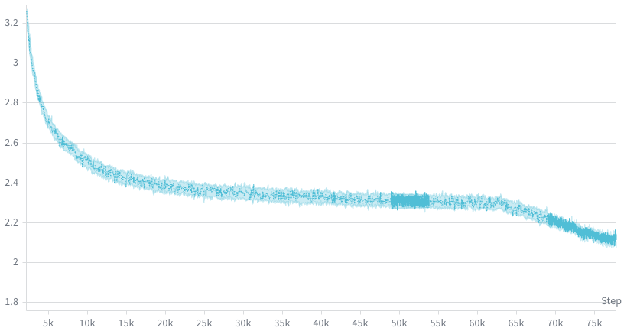
Below is the associated loss curve, which showed zero loss spikes over the 326 billion token run.
An animation of the bias terms used to balance the experts is shown below. Early layers, which are typically much harder to balance, show larger bias terms.
As a comparison point, the animation below shows the routing quality of our prior 1e21 run, which used a combination of a fixed-increment bias term and a small load balancing loss, following a similar convention to Nemotron 3 Super6. Despite also having two leading dense layers, the 1e21 run had a harder time achieving balancing in the first 5,000 steps.
In this 1e21 run, the model eventually balanced to a reasonable level, but the early layers were quite chaotic for the first 5,000 steps, with some experts completely dead for 50+ steps. This left us wondering: should we increase the load balancing coefficient in earlier layers? Should we scale up the bias increment? Should we implement SMEBU and tune the coefficients? What will happen if we scale up 10x? We found that when we later shifted to QB the experts balanced much faster during warmup, giving us confidence to scale up.
Once we've proven out MoEs at 1e23 scale on Marin infrastructure, we plan to look for every 1-2% efficiency gain we can find. For instance, we noticed that layer 4 had a pair of experts consistently running at around 70% of balanced load. This is not a degenerate case (early layers may naturally have different loads across the token space), but there is a possibility we can eke out slightly improved performance here. The current QB implementation is a one-step approximation based on the prior step's routing scores. In future work, we can step through the exact calculations driving the load on these two experts, to understand if there is an update that would pull them back to 100%, or if there is any material impact to the loss curve.
Since QB does not directly push the routing vectors apart, and only adds a secondary bonus term, we also looked at how the routing vectors behave over training. More details on the math of routing vectors can be found in prior work from Google7.
The cosine similarity between each pair of routing vectors is plotted below, which lets us see if any experts are converging to the same routing representation. In the first layer, the expert routing vectors converge around step 4,000, then gradually spread out into their own portions of the vector space by step 60,000. The geometry of the routing vectors in the later layers is less dynamic.
We plan to continue using QB in our MoE runs as long as it keeps giving promising results, and we recommend it to others who are looking for a robust load balancing technique.
The full 1e22 run plotted above is available on Weights & Biases.
The QB implementation in JAX used in this run is available in the Marin repo:
See Anthropic's Toy Models of Superposition for why individual neurons rarely correspond cleanly to single concepts.↩
Li et al., The Lazy Neuron Phenomenon: On Emergence of Activation Sparsity in Transformers, ICLR 2023. Reports as low as 3.0% nonzero MLP activations for T5-Base and 6.3% for ViT-B16, with sparsity emerging naturally across architectures and modalities.↩
Lepikhin et al., GShard: Scaling Giant Models with Conditional Computation and Automatic Sharding, 2020.↩
Wang et al., Auxiliary-Loss-Free Load Balancing Strategy for Mixture-of-Experts, 2024.↩
Singh et al., Arcee Trinity Large Technical Report, which introduces Soft-clamped Momentum Expert Bias Updates (SMEBU).↩
NVIDIA, Nemotron 3 Super Technical Report.↩
Fedus, Dean, and Zoph, A Review of Sparse Expert Models in Deep Learning, 2022.↩
Cite this post
@misc{dial2026_quantile_balancing,
  author = {Dial, Larry},
  title = {Mixture of Experts Quantile Balancing: Validated at 32B-A5B (1e22 FLOPs) Scale},
  year = {2026},
  month = {apr},
  howpublished = {\url{https://www.openathena.ai/blog/quantile-balancing/}},
  note = {Open Athena Blog}
}