In our last post we covered the Delphi Scaling Suite, where we trained dense models up to 1e23 FLOPs. Since then we've scaled up our Mixture of Experts (MoE) recipe to beyond 100B parameters and 1e23 FLOPs and added several architecture and optimizer improvements. This post first covers the MoE transition, then each subsequent improvement, and closes with several promising future directions.
Key terms
- Theoretical speedup — counts only model FLOPs, ignoring MFU.
- Realized speedup — reflects wall-clock time, accounting for MFU.
Speedups are written as theoretical (realized).
Summary
Starting from our Dense Baseline, we achieve the following speedups:
- 6.7× (3.6×) Moving from dense to Marin MoE V1.
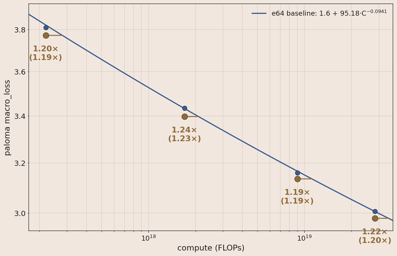
- 1.4× (1.3×) Increasing expert sparsity by raising total experts from 64 to 256.
- 1.3× (1.25×) Updating our optimizer from AdamH to MuonH.
- 1.2× (1.2×) Adding partial key offset (PKO).
- 1.04× (1.04×) Adding routed expert normalization + scaling.
The dense → MoE V1 transition was validated at 1e23 FLOPs. The four subsequent improvements were each measured against MoE V1. We then tested the stacked recipe at 3e19 FLOPs, observing a 2.1× theoretical speedup over MoE V1.
From Scaling Dense Models to Scaling MoEs
The primary goal when we transitioned to MoEs was to demonstrate stability and predictability of scaling to over 100 billion parameters. We incorporated the following techniques to accomplish this:
- Added quantile balancing1 to maintain similar token counts across 64 routed experts per layer, 4 of which are active per token. We detail the impact of QB in an earlier post here.
- Kept AdamH2 as the optimizer, which constrains the matrix Frobenius norms explicitly instead of relying on weight decay.
- Added a light z-loss on the router logits and final logits.
- Added attention gates3 and gated norms4, which reduce outlier activations and give a slight speedup.
- Added Exclusive Self Attention5, which adds another speedup and cleanly lets tokens no-op via a self-attend.
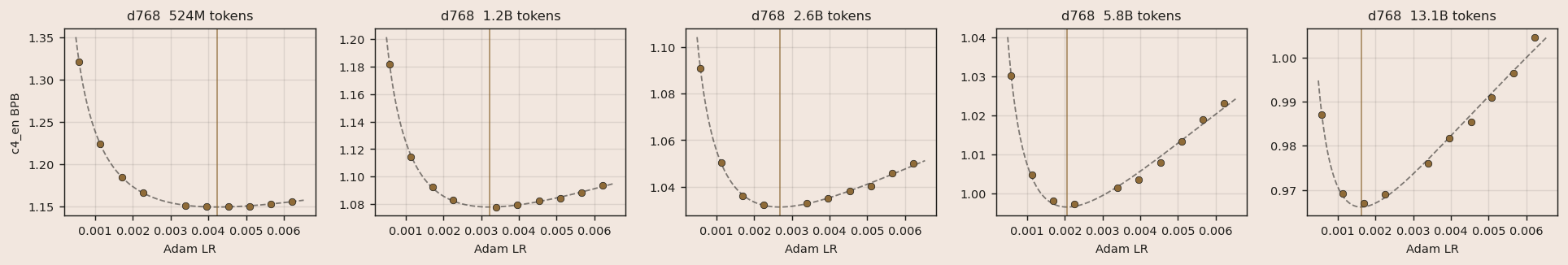
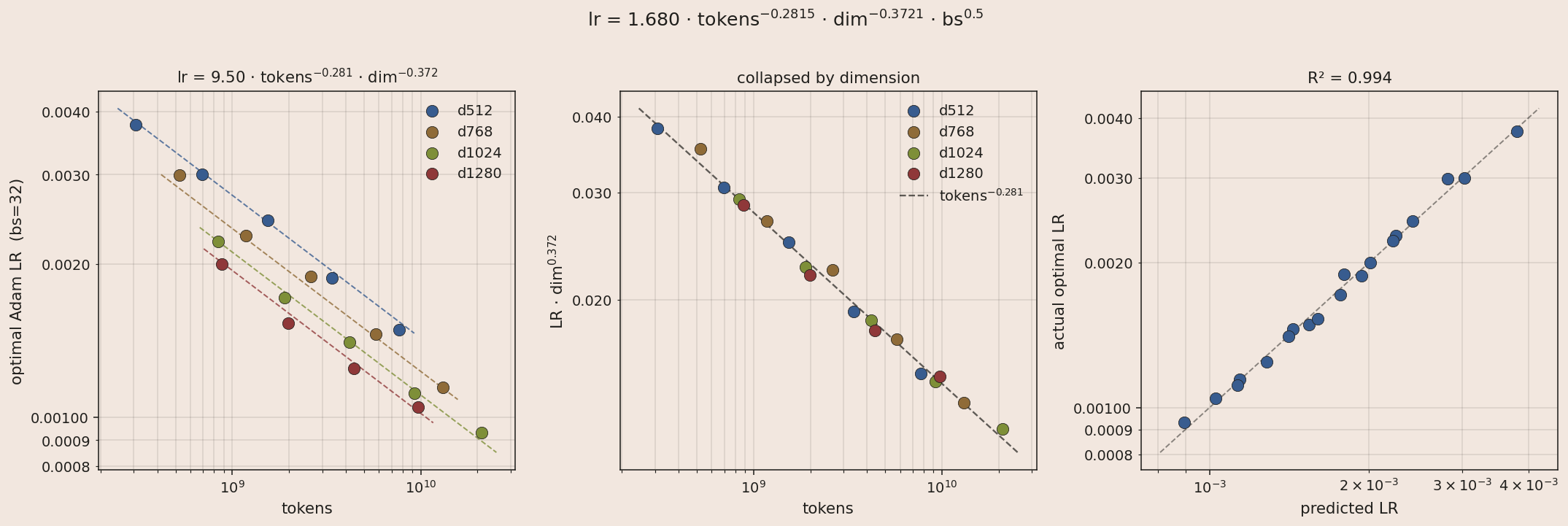
We put extra emphasis on Adam LR tuning, to ensure that future optimizer ablations compare against a tuned baseline. We sweep over model size, token count, and lr in order to fit the form $lr = A \cdot \text{tokens}^b \cdot \text{dim}^c \cdot \text{bs}^{0.5}$, derived in Figures 1 and 2. We scale layer count roughly linearly with hidden dim.
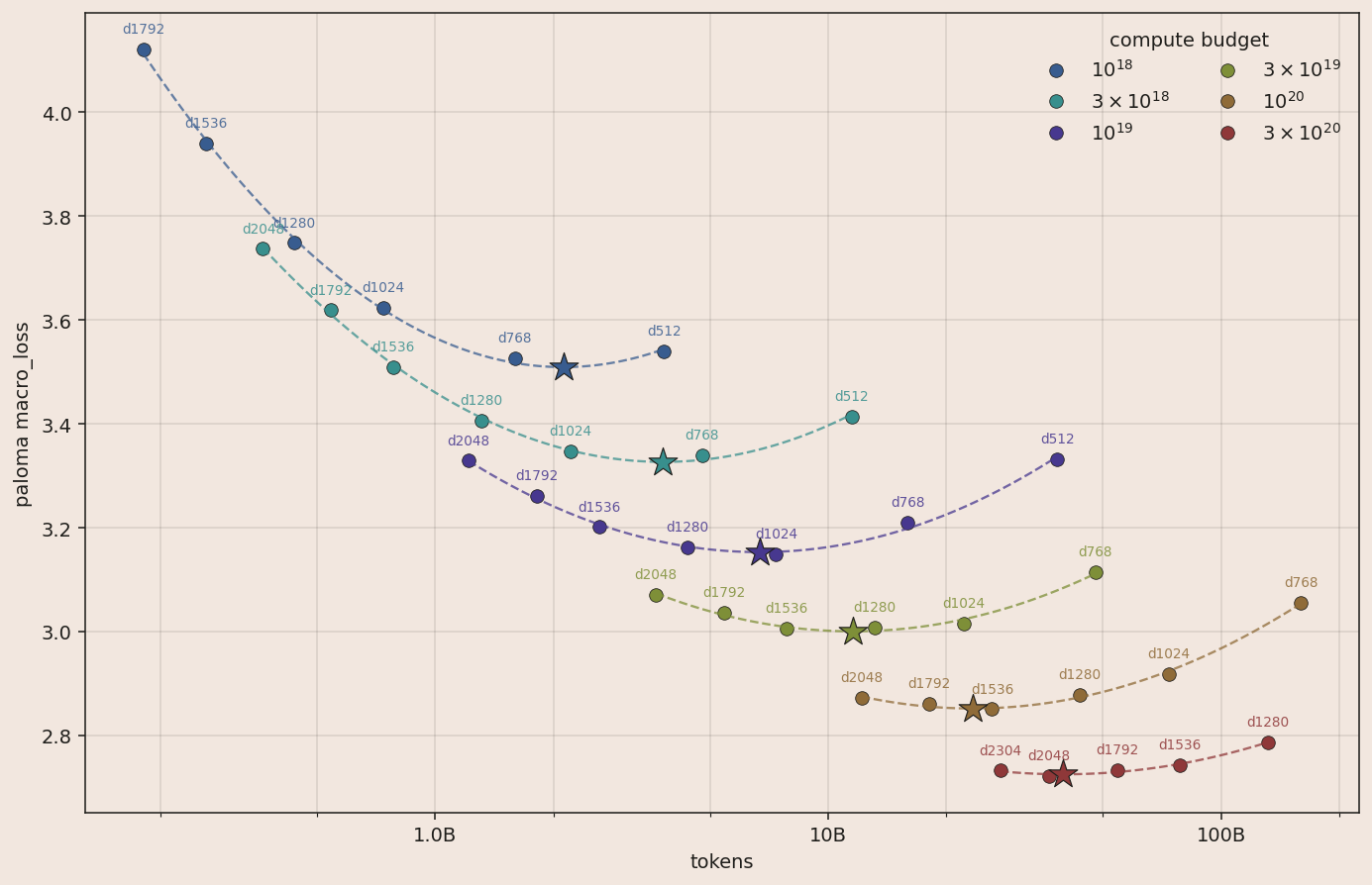
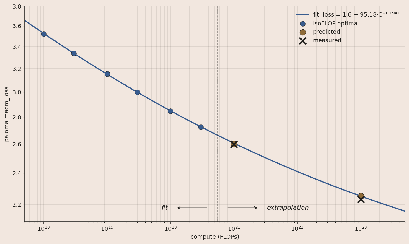
An isoFLOP sweep then gives us an optimal 62:1 token:active_parameter ratio for scaling and a pre-registered loss target for a 1e23 run: a 129B-A16B model trained on 1T tokens, which we call Marin MoE V1.
These choices result in a training run with a smooth loss curve across the entire trajectory.
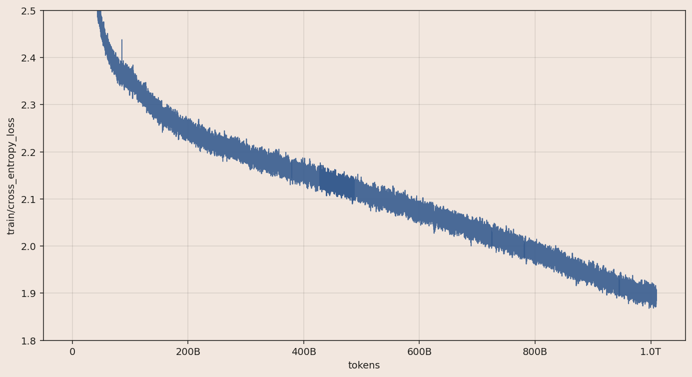
The final loss of the 1e23 run comes within 1% of our preregistered prediction.
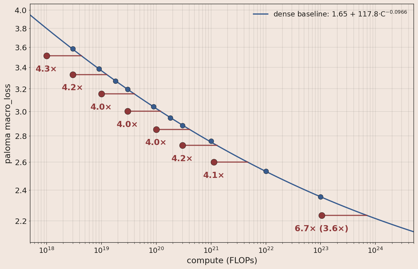
The MoE V1 recipe showed consistent gains over the dense recipe, growing to a speedup of 6.7× (3.6×) at 1e23.
Building on Marin MoE V1
Now that we had demonstrated predictable scaling, we turned our focus to speeding up learning. We assessed changes across 4 compute scales, comparing to the MoE V1 scaling law, with an emphasis on gains that did not diminish at scale. Runs defaulted to the MoE V1 recipe's compute-optimal budgets and tuned learning rates, making the bar for inclusion conservative. We measured loss as cross-entropy across 16 equally weighted Paloma6 categories including code, wikitext, and general web.
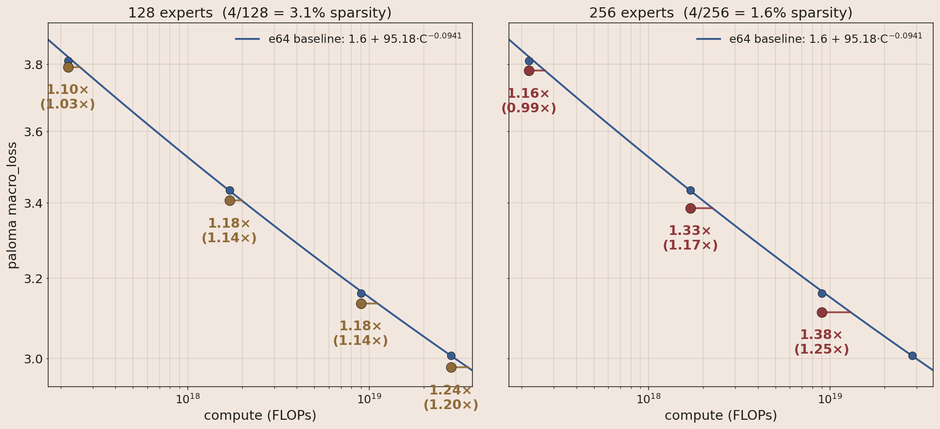
Expert Sparsity
Going from 64 → 128 → 256 routed experts (4 active) shows consistent gains. More experts give the model more capacity to absorb information from the training data, without raising per-token FLOPs.
MuonH
Adam can be loosely described as "take an equal step size on each parameter, then reactively slow down on unstable ones." Muon7 takes a different approach: for each matrix, it orthogonalizes the gradient before applying it, bounding how much that matrix can change its output for any input. One perspective (of many) on why this helps: layer updates happen simultaneously, so each layer's gradient is computed assuming the others are static. If an earlier layer's update substantially shifts the activations flowing into a later layer, the later layer's gradient was estimated against a distribution that no longer exists.
Similar to the baseline, we apply the hyperball wrapper on the matrices and language-model head as a replacement for weight decay.
Partial Key Offset
PKO is a zero-parameter preprocessing of attention keys that gives a 20% gain across all 4 tested compute scales on our evals.
MoE V1 uses Rotary Positional Embeddings (RoPE). Half of the gain of PKO is attributed to partial RoPE, which limits RoPE to only the first half of the head dims on both queries and keys. Before describing how PKO extends partial RoPE, I will first show examples where the PKO model over- and underperforms partial RoPE at 1e19.


The motivation for PKO (first used in modded-nanogpt) is that a single attention layer can't do "retrieve the continuation of X from earlier context": mechanically the query matches on a key at position $t$ but should read the value at $t+1$. Forward-shifting all keys by one position fixes this, but breaks classical "find and retrieve X" attention. Under sliding-window attention with partial RoPE, we observe that pattern-matching inductive behavior emerges in the stationary dimensions of the long-window layers, so we restrict the key shift to those dims on only every 4th layer. PKO's gain is much larger on evals than on training loss, suggesting its pattern matching behavior is more robust to distribution shift.
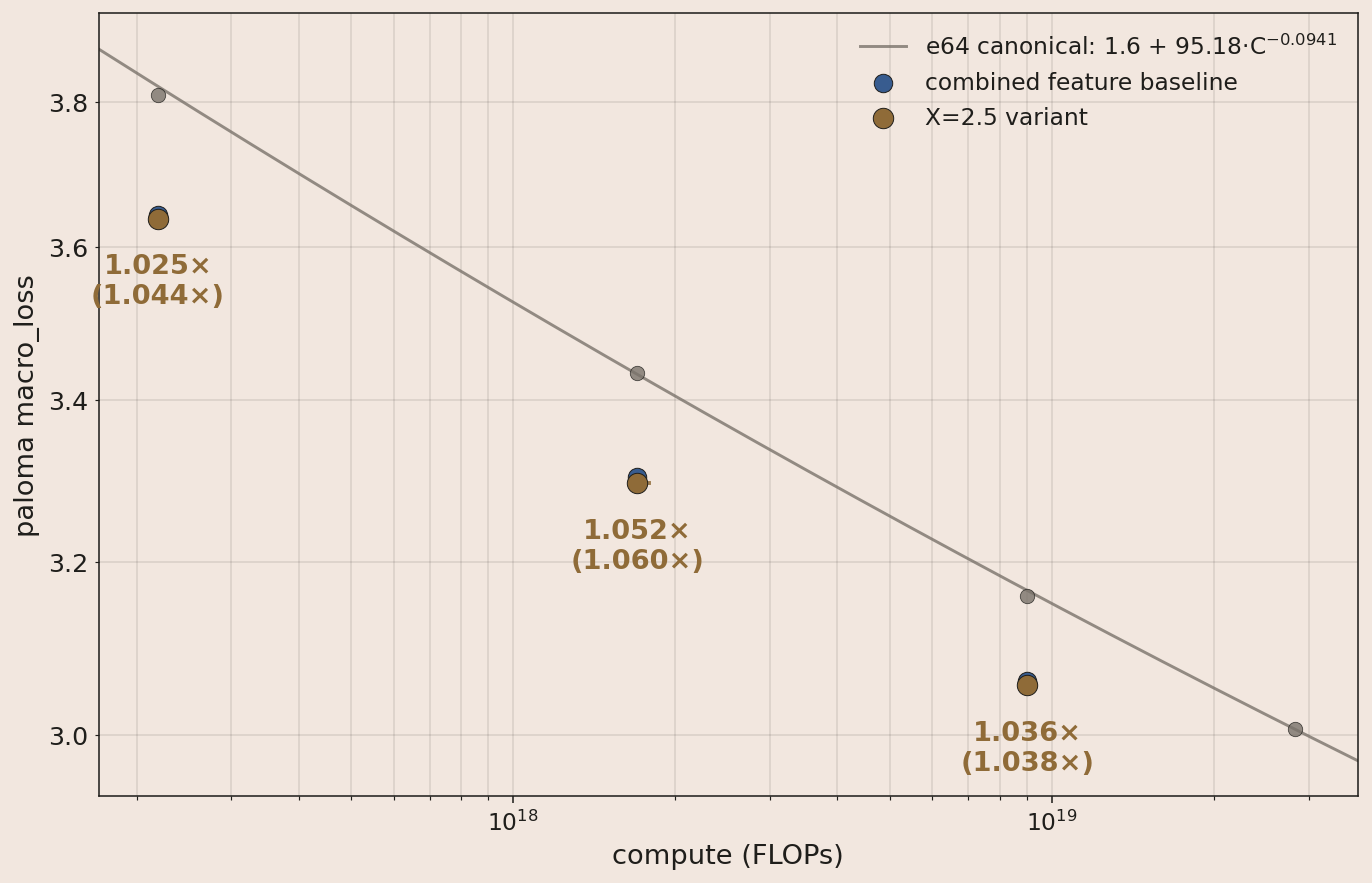
Routed Expert Normalization and Rescaling
Marin is open-development: anyone can follow experiments and contribute. Elie Bakouch, a community member, recently noticed a difference between our expert weighting and DeepSeek's8. Within hours of his suggestion to renormalize and scale the routed expert outputs, we confirmed the small boost and added it to the recipe. Without his recommendation, this improvement would not have made it into our next large scale run. When evaluating the change, we compared to the in-progress recipe indicated by the blue dots below.
Combining all 4
Running the same isoFLOP sweep on the new recipe (solid bowls below) shows the compute-optimal point at each budget shifting to more tokens and fewer active parameters, when compared to the Marin MoE V1 recipe. The shift is likely driven by Expert Sparsity: 4× more routed experts giving the model more sparse capacity to absorb information from extra training tokens.
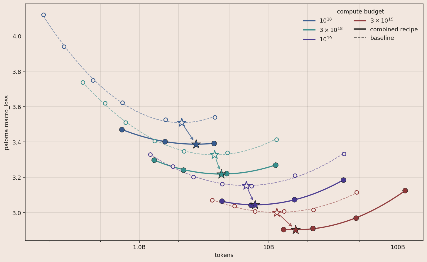
Stacking all four improvements gives a roughly 2× combined theoretical speedup, compared to the Marin MoE V1 recipe.
Recapping the changes:
- Moving from dense to MoE V1 gave a 6.7× (3.6×) speedup at 1e23 FLOPs.
- Treating MoE V1 as the baseline, stacking the four subsequent improvements gives a 2.1× theoretical speedup at 3e19 FLOPs. We don't have data on the exact realized speedup due to shifting hardware mid-experiment, but conservatively estimate it at 1.8×, with slight slowdowns from MuonH and higher expert sparsity.
Promising Future Directions
Residual Bottleneck
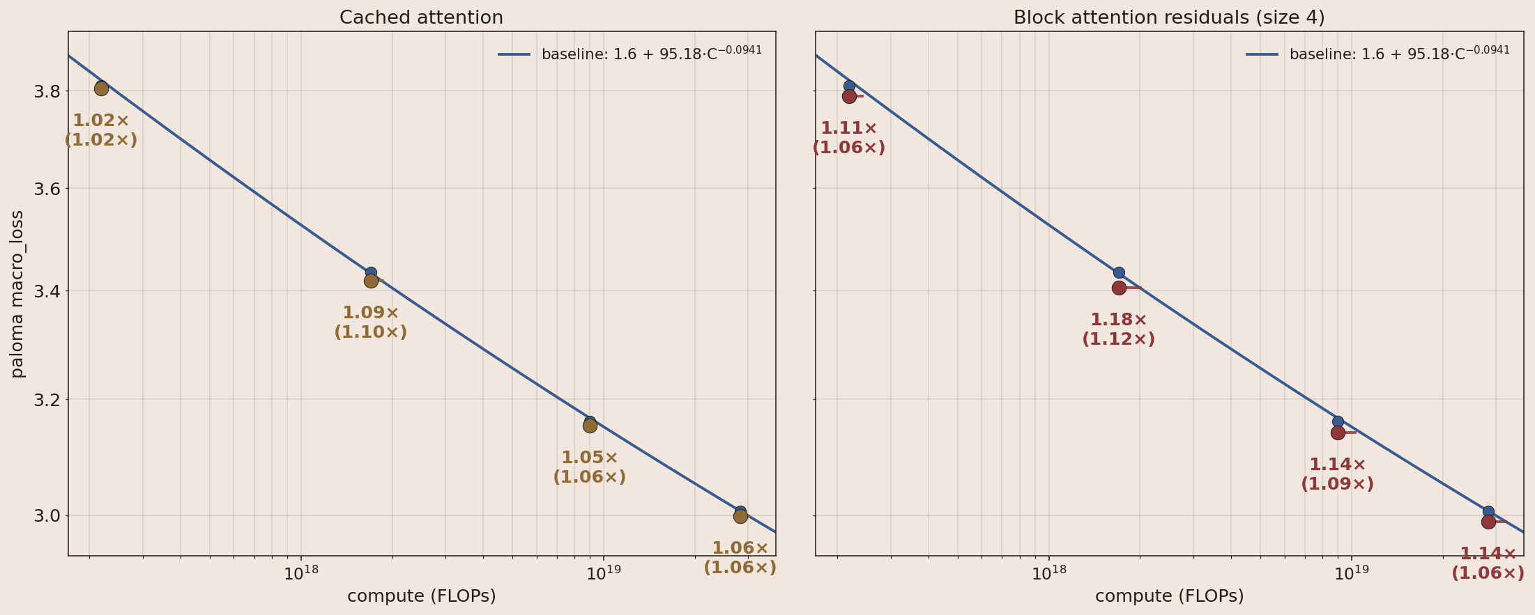
The standard transformer progressively adds to a single residual stream, slowly transitioning it from single token, to token context, to prediction. A large number of techniques have shown improvements upon this, including attention residuals9, per-layer embeddings10, MUDD skip connections11, manifold hyperconnection12, and engram13. Our experiments suggest over 15% speedup is possible, but we're holding off to control the amount of complexity we add to the architecture at each iteration.
A trivial example of caching the residual stream at the 3rd to last layer and feeding it into all subsequent attention modules is shown, to indicate just how many ways it's possible to outperform the standard residual stream behavior. Block attention residuals is included as well.
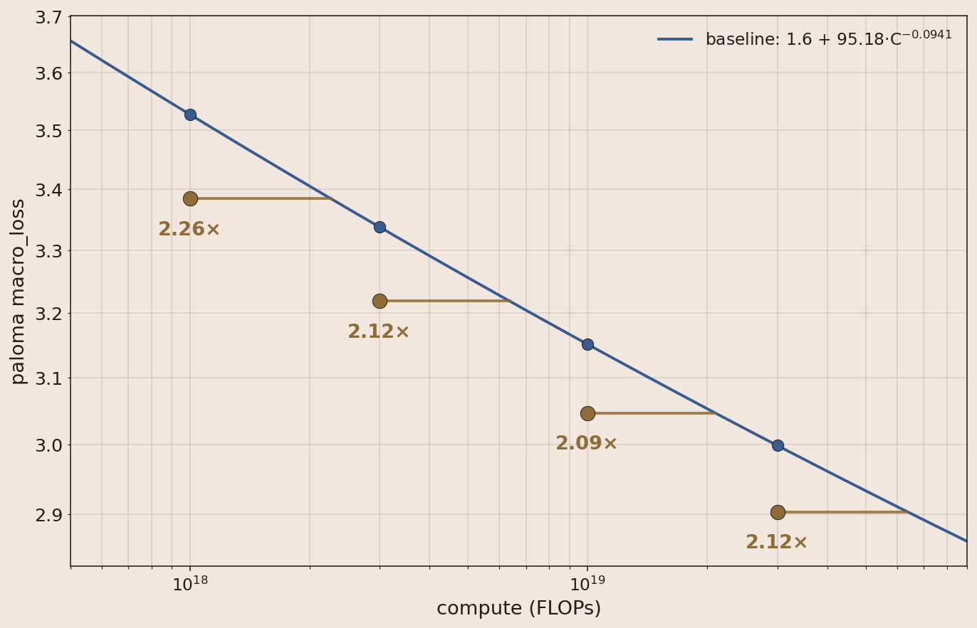
Inference Efficiency
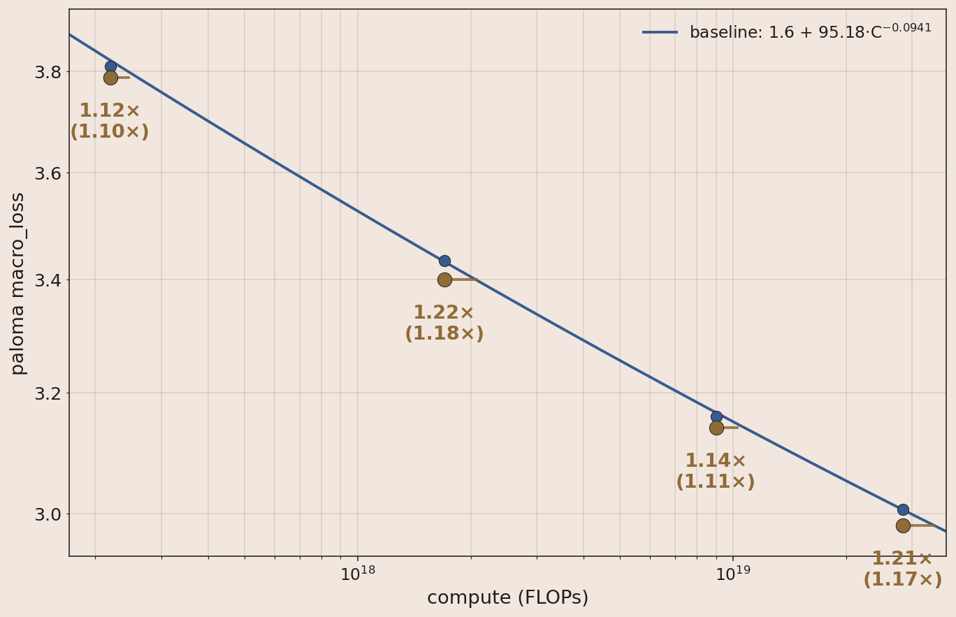
So far the focus has been pretraining intelligence, but another critical axis is inference efficiency, which is important for downstream use and RL. As we grow our RL stack, it will be advantageous to go beyond our current recipe of 4:1 Grouped Query Attention (GQA) with local/global Sliding Window Attention at 3:1 ratio. Promising candidates include multihead latent attention14, gated delta net15, LatentMoE16, multi-token prediction17, and quantization.
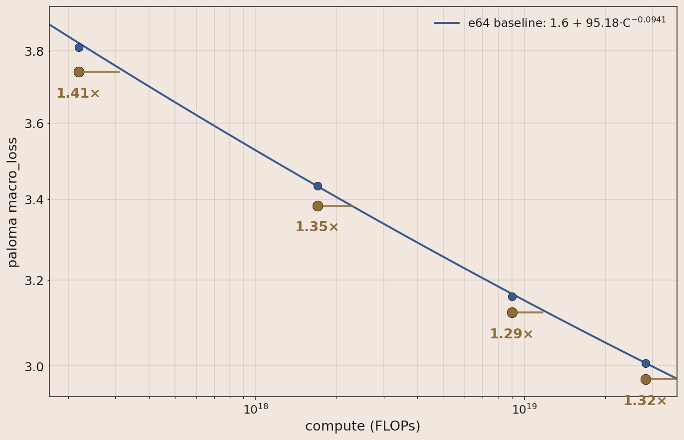
Below: the speedup from reverting 4:1 GQA to full multihead attention. Mechanisms like multihead latent attention may close the quality gap GQA opens while still shrinking the KV cache.
Compute Resources
These experiments were made possible through the generosity of the Google TPU Research Cloud.
Jianlin Su, Quantile Balancing.↩
Wen et al., Fantastic Pretraining Optimizers and Where to Find Them — Hyperball Optimization.↩
Qiu et al., Gated Attention for Large Language Models: Non-linearity, Sparsity, and Attention-Sink-Free, 2025.↩
Qiu et al., A Unified View of Attention and Residual Sinks: Outlier-Driven Rescaling is Essential for Transformer Training, 2026.↩
Zhai, Exclusive Self Attention, 2026.↩
Magnusson et al., Paloma: A Benchmark for Evaluating Language Model Fit, 2023.↩
Keller Jordan, Muon: An optimizer for hidden layers in neural networks, 2024.↩
DeepSeek-AI, DeepSeek-V3 Technical Report, 2024.↩
Kimi Team, Attention Residuals, 2026.↩
Google, Gemma 4 model card.↩
Xiao et al., MUDDFormer: Breaking Residual Bottlenecks in Transformers via Multiway Dynamic Dense Connections, 2025.↩
Xie et al., mHC: Manifold-Constrained Hyper-Connections, 2025.↩
Cheng et al., Conditional Memory via Scalable Lookup: A New Axis of Sparsity for Large Language Models, 2026.↩
DeepSeek-AI, DeepSeek-V2: A Strong, Economical, and Efficient Mixture-of-Experts Language Model, 2024.↩
Yang et al., Gated Delta Networks: Improving Mamba2 with Delta Rule, 2024.↩
Elango et al., LatentMoE: Toward Optimal Accuracy per FLOP and Parameter in Mixture of Experts, 2026.↩
Gloeckle et al., Better & Faster Large Language Models via Multi-token Prediction, 2024.↩
Cite this post
@misc{dial2026_pretraining_speedup,
  author = {Dial, Larry},
  title = {Improving our LLM Pretraining Efficiency},
  year = {2026},
  month = {jun},
  howpublished = {\url{https://www.openathena.ai/blog/pretraining-speedup/}},
  note = {Open Athena Blog}
}